Previously, we — the Data Science Campus at the Office for National Statistics — created blog posts on how to use our Google Data Studio Community Visualisations choromap and choromap-lite. Both tools have been very successful, not only for projects we run at the Data Science Campus, but also for others around the world looking for a choropleth map solution to their Data Studio visualisation needs. Since releasing these tools, we have spoken to people around the world on how to use choromap and choromap-lite. We have also incorporated outside collaborators’ improvements via our GitHub page.
Until now, the choice of whether to use choromap or choromap-lite depended on the user’s needs. choromap-lite is useful for small GeoJSON files and time series data; whereas choromap can handle larger GeoJSON files.
However, in this post, we show how the heavyweight choromap can use Google Data Studio’s Blend to:
- improve run-time and efficiency when displaying time series data, and
- allow the user to change the GeoJSON boundaries displayed.
That is, the user could view data at a national level, then switch to exploring the data at a more granular level. With choromap you can put the power of data exploration on choropleth maps in the hands of your user.
1 Why not just a BigQuery join?
Suppose we have a time series data set comprising multiple geography levels (we call this the Metric data set). Each geography area has a single data point for each day of the week. The total number of data points is n x m, where n is the number of polygons in all geography levels and m is the number of days. On its own, this data set may not be large. For a time period of around two weeks the data may only be 1 MB or less. However, the Geometry (GeoJSON) data for all these polygons may be considerable larger, at around 10 MB for even the most generalised shapes (we call this the Geometry data set). If we joined those two data sets together so that each data point had a geometry cell (as required in choromap) our resulting table would be over 200 MB in size. This is because of the replication of the geometry information for each time series data point. For a year’s worth of data, this would be several GBs of data when joined.
 Figure 1: An image showing a sewing machine
Thus, by joining the two data sets, all we have done is make a larger data table before it has been passed to Data Studio and choromap. A useful thing about Data Studio is that metric aggregations are done before the data is passed to a Community Visualisation like choromap. So, what if we could only load the Metric and Geometry data we want to visualise and then join the filtered data sets?
That’s where blending in Data Studio comes in.
2 Data Studio Blend
Before blending, both Metric and Geometry data sets need to be added to the report. After which, choromap needs to be added from the Community visualisations and components menu. When they are added, the Metric and Geometry data sets can be blended by clicking (+) Blend Data below data source on the right-hand side when editing the choromap widget. In the first column, the Metric data set can be selected; the second column can then comprise the Geometry data set. The number of join keys depends on whether the Metric data set comprises multiple geography levels. If it is a single geography level, then the join key can just be the unique area ID, common to both data sets; if the data comprises multiple geography levels (national, county, city etc) then the join key should be the unique ID and a field specifying the geography level. This is because in some cases different geography level areas may share the same code, e.g. a county which is also a city. Finally, the relevant dimensions and metrics can be included in the blend.
3 COVID-19 Cases Example
COVID-19 cases data is an ideal example of time series data presented at multiple geography levels. The UK Government make a number of statistics available for the general public at coronavirus.data.gov.uk. Here, we have used their API to download COVID-19 case data (by specimen date) for the time period 1st January 2021 to 15th January 2021. We have also downloaded the data for the UK, each UK nation (England, Scotland, Wales and Northern Ireland) and for each English region (London, East of England, South East, Midlands, North West, South West, and North East and Yorkshire).
Disclaimer: this is a cut of official data and our use here as part of the Office for National Statistics is purely for visualisation purposes and not to comment on the data or trends.
The downloaded COVID-19 case data was uploaded to Google BigQuery alongside a GeoJSON CSV file comprising the geometries for each geography level. These geometries were downloaded from geoportal.statistics.gov.uk, converted to WGS84 reference system using QGIS and then saved as a CSV as shown in Section 1. Data: Fitting a square peg in a round hole of this blog post. Both data sources were added to a Data Studio report and then blended, as shown below.
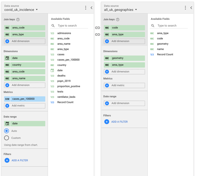 Figure 2 An image showing how the two data sources were blended
choromap can then use the geometry information from the Geometry data set and the data from the Metric data set to create the visualisation. You can then filter the data based on a date and/or the geography level you’re interested in. The final result is shown below in a GIF.
 Figure 3: A GIF showing how the user can choose different dates and geography levels to present the data at on a map
We have shown in this post how we can use Google Data Studio’s Blend functionality with choromap to make engaging and dynamic choropleth maps. A report for this work has been created here.