While working on the urban forest project, I created a tool to visualise some of the project’s output data.
This city profiler is just one example of how the urban-forest data can be used. Specifically this app makes it easy to see how much urban vegetation certain areas have at both the parish and street level. While currently the app only shows the Urban Forest data, it would be possible to add any other data on a given area, making it easier to see the potential relationships between urban vegetation and other factors. For example it may be interesting to compare a particular area’s urban vegetation with house prices, or levels of deprivation. While there are likely to be complicated relationships involving much more than just these two variables, it is none the less interesting to be able to clearly visualise and aid in identifying particular areas of interest.
The web app uses a small section of the total urban-forest data, focusing on Cardiff. This is not only interesting for me as I live in Cardiff, but was also a great learning experience to try building an interactive shiny app. As well as the shiny app, I created a package, gRoot, to host the app, data and functions. This keeps the UI and Server of the app more readable by keeping larger functions out of the main body of the app. In this post, I’ll give a brief run through of the process of this project and what I learned along the way.
The app
This web app is built in shiny, an R package that makes it easy to build dashboards or other ways to visualise data. Within the app I have used leaflet, a JavaScript library for creating interactive maps. Leaflet has an R package that integrates with shiny really well, allowing easy manipulation of the leaflet map by shiny elements and vice-versa. This interaction will be mentioned throughout the post. As well as leaflet and shiny, I have made significant use of libraries such as ggplot2 and dplyr for visualisation and data manipulation respectively. Learning these tools has proved to be incredibly useful for a number of other projects that I have worked on since.
Data
I only required two datasets for this app, the urban-forests point data and a geojson of polygons. The method that I used could be used on any geography with an available geojson file, however I chose to use parishes as most people know which area of the city they live in and probably don’t know their LSOA code!
Geojson manipulation
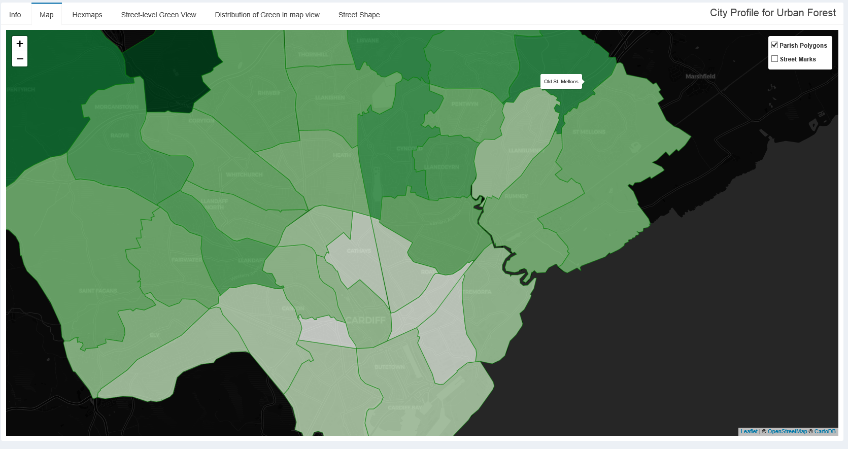
The first stage in this project was manipulating the data so that it could be easily visualised on a leaflet map. At this stage, there was no shiny app, just a leaflet map. In this initial phase I had the polygons of the Cardiff parishes in geojson format and the points in a dataframe in csv format. To colour the parish polygons correctly, I developed a function to find which points fell into which polygons and then take an average of these points. Fortunately R has a number of packages for manipulating geojson files such as geojsonio and sp. Using these packages, I created three functions: one to convert the geojson of points to a dataframe, another that finds which points fall in which polygon so that each point can be given a parish, and finally a function that takes the points that fall within a polygon to create a summary statistic for that polygon. I will note here that each point has two figures for vegetation, one of the left and one on the right. I chose to report the maximum value of vegetation for each point, and is worth bearing in mind when using this visualisation.
When each parish polygon had a mean green value, I varied the fill colour for each polygon by this value. This makes it immediately obvious where the areas of Cardiff with the most urban vegetation are. There are issues with this however. Take Tongwynlais as an example; there is only one road recorded here which has a high level of urban vegetation. While it is likely a very green area, we can’t know if the other roads in this parish are as green as this method appears to show.
A basic Shiny App
Once the map was working and polygons were layered over the top, coloured to
their corresponding level of urban vegetation, I built the shiny app around the
map. A shiny app comprises of a user interface (UI) and a server. The UI holds
all the code controlling the arrangement and organisation of various elements,
while the server controls those specific elements and interactions between them
using a reactive
framework. In this app I have split the UI and the server into different
scripts; decoupling is good practice when working in a team as it allows
different members to make changes to the UI and server simultaneously. The
function runApp() will look for a UI.r and server.r in the current working
directory.
I won’t go into detail on how to create a shiny app here as there are already many tutorials that clearly explain how to design a shiny app.
The initial app simply contained the leaflet map with a title panel. Structuring a shiny app is very easy, making it simple to add new components or interactions when you need to.
Distribution and summaries of Urban vegetation
Following this, I wanted to be able to look at the distribution of levels of
urban vegetation in any chosen area. I found that input$map_bounds provides
coordinates for the top left and bottom right corners of the view of the map.
Using these values, I could easily subset the data and create a histogram of the
urban vegetation with this subset.
I created a function that allows you to subset data by a set of coordinates, which I found that I was doing often throughout this project. Again this is stored within the gRoot package.
I used the same approach to create a summary table, but varied what was
displayed by the zoom level. This was available from input$map_zoom.At a high
zoom level, summary values at the parish level are shown while at lower levels,
street summaries are shown. Functions for both the table and the histogram are
found in gRoot. Housing these functions within a package has two key benefits.
Firstly, as already mentioned, it keeps the server script a bit cleaner and
easier to read. Secondly, should I want to use the function outside this shiny
app, I can simply load the package and the function is available for me to use.
Urban vegetation by Street
Once I had urban vegetation at street level I wanted to look at how urban vegetation varied through those individual streets. There were a number of stages to this which I will break down here.
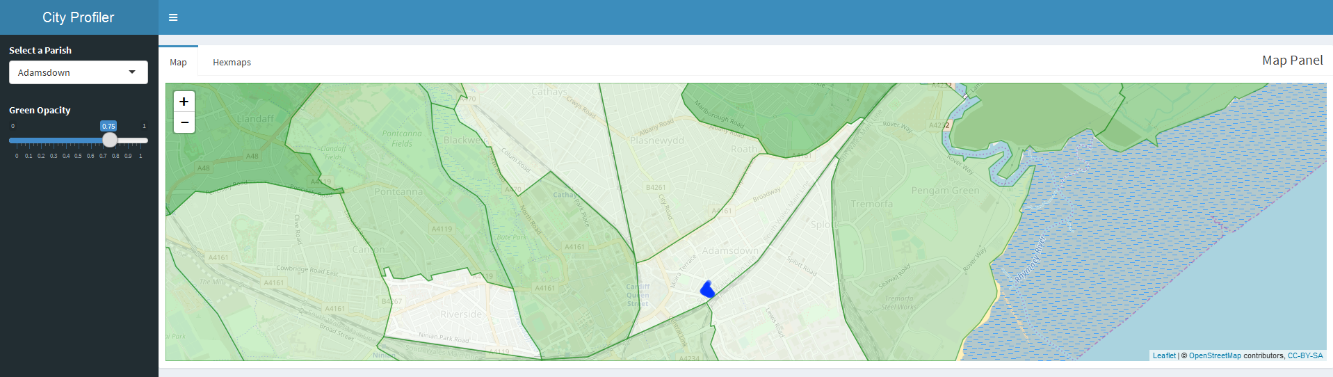
Selecting the streets
To select the street I subsetted the data by parish, using a drop-down to select parish. This was simple to do by passing the character vector to the choices argument of input_select. The street names are included in the urban forests data set. As mentioned in the manipulating geojson section, I had attached a column to this dataframe with the parish for each recording. Note that this means that some streets will show up in multiple parishes. Next I created a second drop-down of streets within the selected parish. I subsetted by parish first as otherwise you are left with a lot of records to sort through to find the street you’re after.
Upon selecting a street, three things should happen:
- A plot of urban vegetation along the street should be shown below the map
- Markers highlighting the selected street should be placed on the map
- Any markers highlighting other streets should be removed from the map
I later added a second street drop-down menu, allowing the user to compare two streets within the same parish.
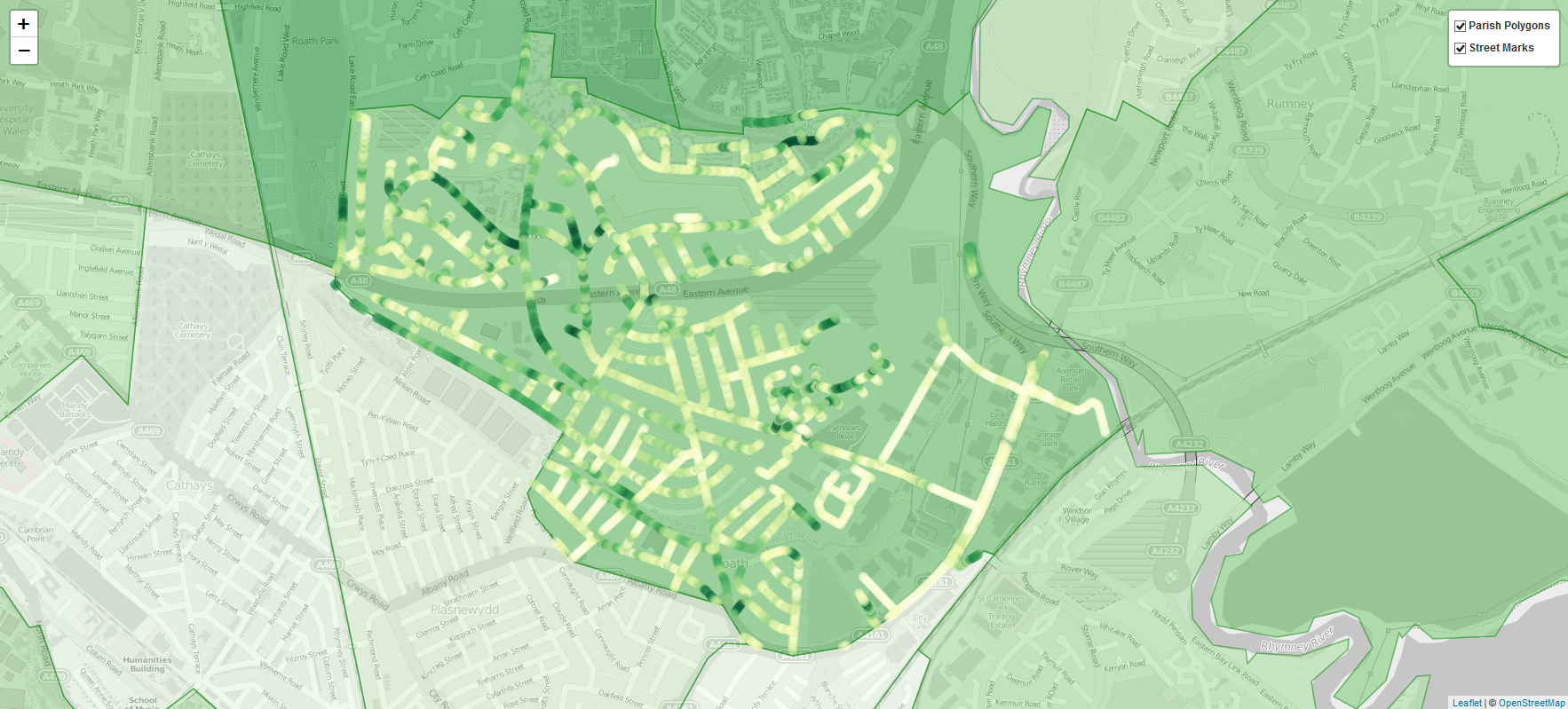
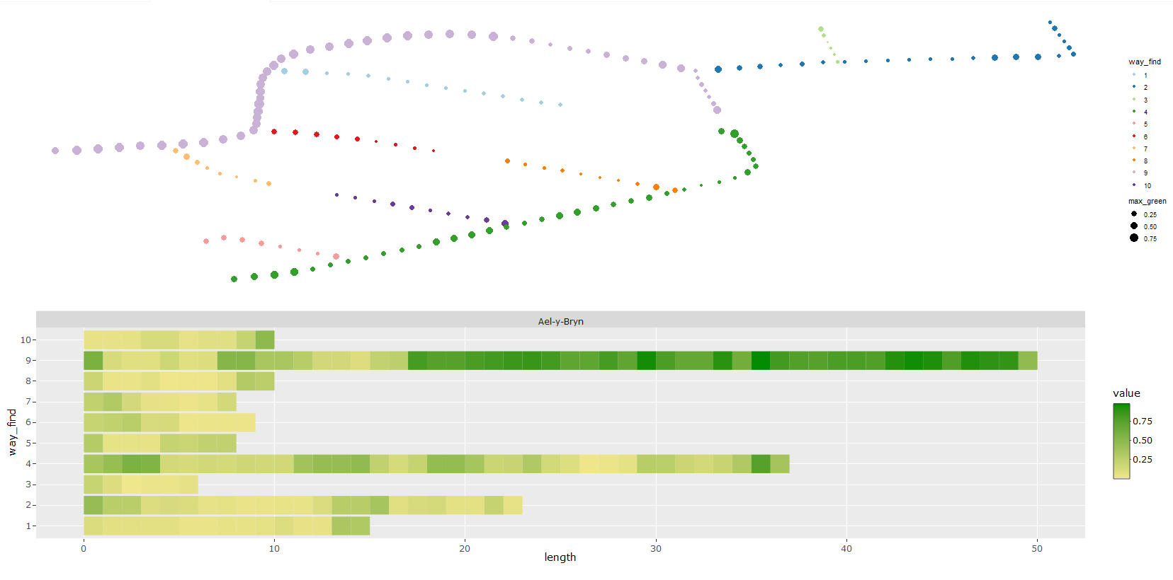
Plotting urban vegetation along the street
This has presented a significant issue. Due to the fact that streets are not
straight, it has proved incredibly difficult to make a single 2D representation
of vegetation along a single street. I opted for a split view that would show
the shape of the street on the along the top of the window by plotting each
point on that road and a plot of vegetation along each way_id across the
bottom. A new way_id will be used when there is a significant branch in the
street, so gives us a work around for plotting streets as straight lines. Each
way_id on the selected street will be shown in a different colour, with the size
of the point giving an impression of the level of vegetation at this point. This
is not ideal, and is something we’d like to improve upon in the future.
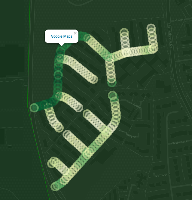
Markers highlighting the selected street
Markers are placed on the map in response to the street selector. Leaflet proxy is generally used for interactive elements that will be placed on a leaflet map. Using leaflet proxy stops the map from being redrawn every time you want to add or remove markers. The snippet below is an example; when the parish select input is active, it then resets the markers that will be placed. Note that in this case, it is important to remove the previous markers prior to adding new ones.
To create the markers, I subset the data by the street name in street selector. For each marker it takes the longitude and latitude of each recording in the resulting subset. Next, it names the marker as the street name followed by the recording number. Finally a popup option is given - when the marker is clicked, a link pops up which contains a URL Google street view of those coordinates. The link is created by taking a standard Google streetview URL and pasting the latitude and longitude numbers into the correct position. The markers all added to a specific layer of the leaflet map; this is important in the next stage of removing the markers.
 .
.
Removing old markers
This step actually occurs before placing any markers. Each time a new street is selected, all previously placed markers are removed before placing new markers. Both responses are controlled by the street selector, but the removing is programmed to happen first. As mentioned in the previous section, markers are added to a specific layer of the leaflet map, meaning I can select to remove the entire layer.
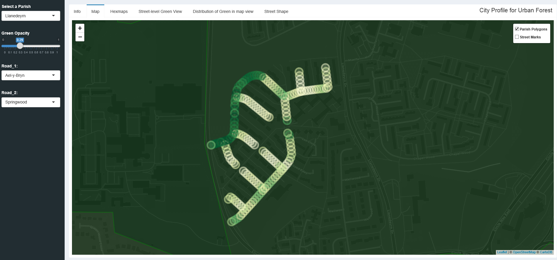
Highlighting all streets in parish
While this is quite visually pleasing, it also provides a useful way to
highlight the greener areas of the parish easily. Like the street specific
points, these all contain a URL leading to Google streetview. Rather than adding
this as an option in the shiny interface, this is controlled entirely by the
leaflet map, and is passed as a layer. This saves us from cluttering the
interface. There is also an option to remove the polygon colours from the map,
though the borders will remain. This did cause an issue initially; because these
are layers, if you add the polygon layer after the markers, then you will not
be able to click on the markers as the polygons lie on top of them. To solve this
I used addmapPane() which came in version 2.0.0 of leaflet. This allows you to
assign levels of mapPanes and to assign components such as polygons and points
to these panes.
gRoot Package
As I’ve already mentioned, learning how to build an R package was another useful skill I gained during this project. There are a number of useful online resources that I used to understand the process, particularly this one. Building a package involves not only designing and organising the functions but also documenting what the functions do, the inputs that are required, what output values to expect and any parameters that can be changed. There are a number of helpful features and libraries in R to make this process easier, Phil pointed me to roxygen, which is a great package for formatting documentation and integrates with R studio. You use specifically formatted comments around your functions and then roxygen creates the Rd. document files for you. It will also create a namespace file.
Within the package I have also included all the data required to run the shiny app. This reduces the requirements for loading datasets in certain folders, as the data will be loaded straight into the environment. It also allows us to update the datasets if required and ensure that the same data is always being used in the app.
The app is now held within the gRoot package, so that by loading the package,
you can run a single function and the app will launch in a browser window.
library(gRoot)
launch_app()
This was done by placing the ui.R, server.R, global.R and associated files
in the inst folder of the package. I then included a function within the package
that calls the shiny::runapp() for that location. By housing the app within
the app, it makes it easier to add new features and fix bugs.
The app is also hosted on datasciencecampus.shinyapps. Hosting the app on shinyapps.io is an easy process, a tutorial can be found here. When preparing to publish an app to shinyapps.io it is worth remembering that you cannot use packages you have developed unless they are hosted on CRAN - at time of writing it is not possible to install packages using devtools::install_github(). All this means is that you will need to edit your global.R file to source any datasets or scripts that contain functions directly.
Looking forward
This app is by no means perfect, but gives an example of what can be done with the urban forest data. One huge improvement that could be made to this would be to include additional datasets such as the Welsh Index of Multiple Deprivation
We’re also looking at collaborating with the Visualisation team to improve the way that we visualise certain aspects of the app. In particular, we would like to implement a clearer and more intuitive feeling of how green a street is as you walk along it.
All code for both the app and the package, as well as the data, will be available in a GitHub Repository.
References
The ggmap package is used in this project, with thanks to the authors below.
D. Kahle and H. Wickham. ggmap: Spatial Visualization with ggplot2. The R
Journal, 5(1), 144-161.
URL: https://journal.r-project.org/archive/2013-1/kahle-wickham.pdf
The “R packages” book was also incredibly useful: https://r-pkgs.had.co.nz/
Finally for packaging the app, this article from Mango Solutions was very helpful.