In this blog we describe how we remove personal information (vehicle number plates) from streamed traffic camera images, in accordance with ONS’ ethical and privacy standards. We are only interested in aggregate, non-identifiable time series, so removing identifiable information is the first part of our processing.
We focus on the process of removing legible and disclosive number plates from downstream processing as part of the Traffic Cameras project published by the Data Science Campus in September 2020. The Traffic Cameras project emerged from the need to better understand changing patterns in mobility and behavior in real time in response to the coronavirus pandemic (COVID-19). The project utilizes publicly available traffic camera imagery, deep learning algorithms, and cloud services to produce in almost real time counts of pedestrians and vehicles in select city centres. Although traffic cameras are not designed to capture number plates, in rare circumstances they may be legible in camera imagery. To prevent us accidentally capturing identifiable number plates, we employ an image downsampling method to reduce image resolutions and therefore detail, which obfuscates number plates in any processed images.
This blog details how we evaluated the impact downsampling had on the performance of object detection algorithms through the assessment of object count time series, where we wished to ensure the time series was of sufficient quality whilst obfuscating number plates. This concludes development work and we have now released the source code to GitHub under the “chrono_lens” repository.
Identifying legible and disclosive example number plates
Collecting, storing, and processing traffic camera images of public spaces poses significant challenges. Our focus here is the accidental disclosure of vehicle registration number plates. The images we collect, store, and analyze are captured at various cameras settings, locations, illuminations and weather conditions. Of the thousands of images recorded at 10-minute intervals, a proportion of which are high definition. Being able to definitively recognize a number plate from these images is rare given that numerous factors must coincide at the same time. Such factors include:
- Camera resolution.
- Number plate angle and distance relative to the camera.
- Speed of the vehicle.
- Weather conditions (rain, fog, and/or sun glare).
While all these factors aligning perfectly is rare, our continuous sampling means we may record dozens of such disclosive images daily. To address this issue, we proposed downsampling all images upon being downloaded that exceeded a given resolution threshold. We had to consider what resolution would suffice to remove all disclosive number plates and secondly measure the impact downsampling images would have on the performance of object detection algorithms and thus object counts.
Downsizing too aggressively would have a needlessly detrimental impact on objects counts. Therefore, an optimal resolution threshold had to be determined. Figure 1 illustrates modified examples of disclosive vehicle number plates recorded on public traffic cameras.
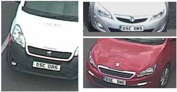
Figure 1: Three modified examples of disclosive number plates captured by public traffic cameras (where the original number plate has been replaced with “ONS DSC”)
Measuring the distribution of image resolutions
We assessed the resolutions of downloaded images aiming to identify the frequency of high-resolution images. Furthermore, we could identify specific locations supplying higher resolution images. To achieve this, for a 24-hour period we recorded the meta data of images provided from all our traffic camera images providers including Transport for Greater Manchester (TfGM). We specifically recorded each image’s width, height, location, and camera ID. Figure 2 illustrates the resolution of images from TfGM, in addition to the number of observations for each resolution.
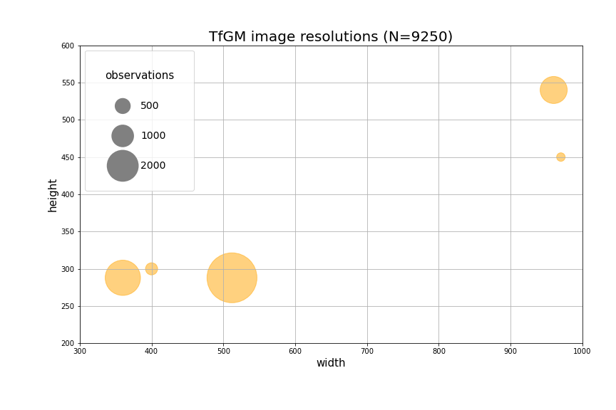 Figure 2: TfGM traffic camera images resolutions and number of observations
Figure 2 shows that a noticeable number of images have widths approaching 1000 pixels and heights approaching 450 and 550 pixels. We see that higher resolution images account for a good proportion of total images. Number plates shown in figure 1 are all sourced from similar higher resolution images. The greater number of higher resolution images increases the probability of recording legible vehicle number plates.
Downsampling images
Applying the same methodology to create Figure 2, we recorded resolutions of images for all available locations noting that the most common image width was 440 pixels. Given that no legible number plates had been identified with images of 440 pixels width, 440 pixels in width was chosen as our threshold to deem an image as being of ‘too high resolution’ if exceeded.
We decided to choose a 24-hour period from all locations to run our downsampling code on. These sample 24-hour periods would later be the subject of our before and after downsampling object count time series analysis. However, choosing a random 24-hour periods would not suffice. Traffic camera ‘uptime’ varies significantly by location, and even week-to-week for any specific location. Luckily, the team had previously developed scripts that recorded the ‘uptime’ of cameras for a given location to accompany our weekly faster indicators release. We could use the output charts to identify healthy weeks and subsequently 24-hour periods to run our analysis on.
Figure 3 illustrates what percentage of images for a given location were recorded as faulty, missing, or present. We see that Northern Ireland and TfGM images recorded greater than 90% of images being present. Conversely, Durham images shows greater than 50% of images as faulty, approximately 20% and 25% as missing and present, respectively. The week ending 27 December 2020 (2020-12-27) is likely a viable candidate from which to choose a 24-hour period for Northern Ireland, TfGM, and Transport for London (TfL).
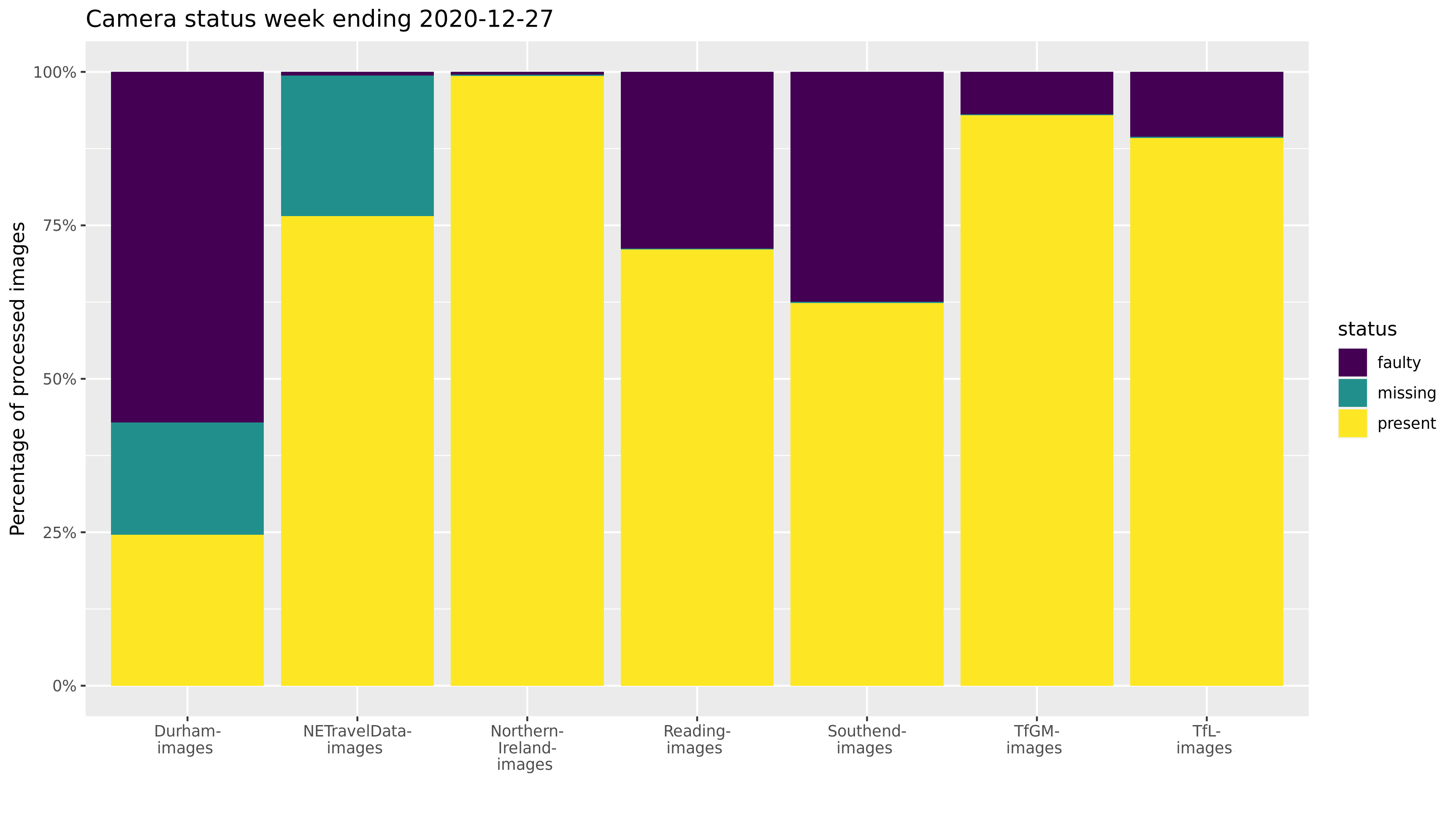 Figure 3: Cameras status report per location for week ending 2020-12-27
Next, we had to assess 24-hour periods within a given week to find the healthiest 24-hour period. Figure 4 shows one week of data identifying periods where individual cameras were either present, missing, or faulty. For TfGM, we see the 22nd of December 00:00 – 23:50 was a healthy 24-hour period. This process of selecting healthy 24-hour periods was repeated for all locations to determine a best possible 24-hour period to conduct our analysis on. Table 1 shows the chosen 24-hour periods per location.
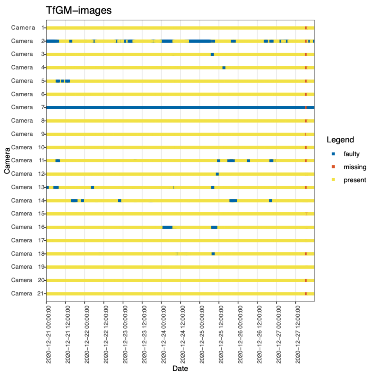 Figure 4: Camera status per camera for TfGM week ending 2020-12-27
| Location | Candidate week ending | Chosen day |
|---|---|---|
| TfGM | 2020-12-27 | 2020-12-22 |
| Northern Ireland | 2020-12-27 | 2020-12-24 |
| North East | 2021-01-10 | 2021-01-05 |
| Durham | 2021-01-17 | 2021-01-05 |
| Reading | 2020-12-27 | 2021-12-23 |
| TfL | 2020-12-27 | 2020-12-22 |
| Southend | 2020-12-27 | 2020-12-22 |
Table 1: Identified 24-hour periods of good camera uptime for each location
Lastly, we ran an iterative script which duplicated 24-hour periods, with higher resolution images (width exceeding 440 pixels) being downsampled to 440 pixels width. Figure 5 shows number plates before and after downsampling, where we employed the OpenCV ‘resize’ function with the interpolation method set to ‘INTER_AREA’.

a. Before (1920x1080) and after (440x274)
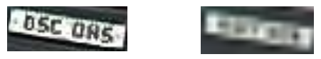
b. Before (1280x1024) and after (440x352).

c. Before (1280x1024) and after (440x352).
Figure 5: Comparison of number plates before and after downsampling
Time series comparison before and after downsampling
Using the meta data described above in the Section ‘Measuring the distribution of image resolutions’, we gathered lists of ‘guilty cameras’ that were known to provide higher resolution images. The lists of ‘guilty’ cameras allowed us to only analyze object counts for images provided by higher resolution cameras. This method served two purposes, (1) to reduce processing time having to only analyze a portion of images instead of the whole collection, and (2) allowed fair before and after object count comparisons between locations as including lower resolution cameras, which make up the majority of images, would bias the result if included. Figure 6 illustrates a 10-period moving average of summed object counts from ‘guilty’ cameras for each 10-minute snapshot for before and after downsampling per location over 24-hour periods. Reading and TfL are excluded from Figure 6 as no cameras from these locations provided images that exceeded our high-resolution threshold.
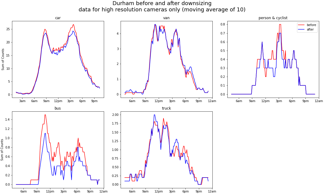
Figure 6a: Summed object counts from ‘guilty’ cameras for each 10-minute snapshot over a 24-hour period before and after downsampling for Durham with an applied 10 period moving average
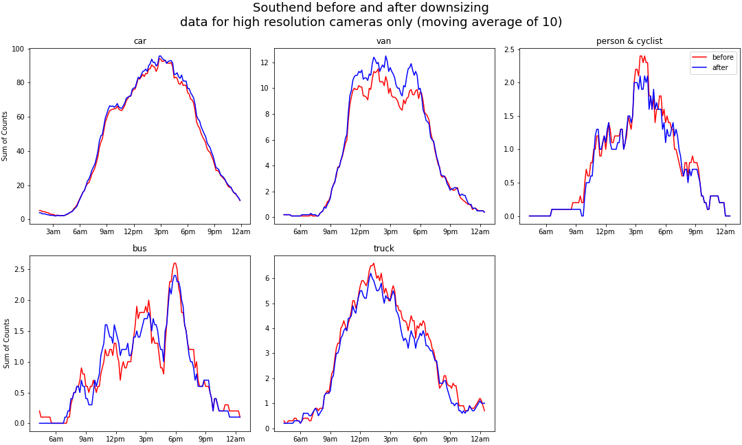
Figure 6b: Summed object counts from ‘guilty’ cameras for each 10-minute snapshot over a 24-hour period before and after downsampling for Southend with an applied 10 period moving average
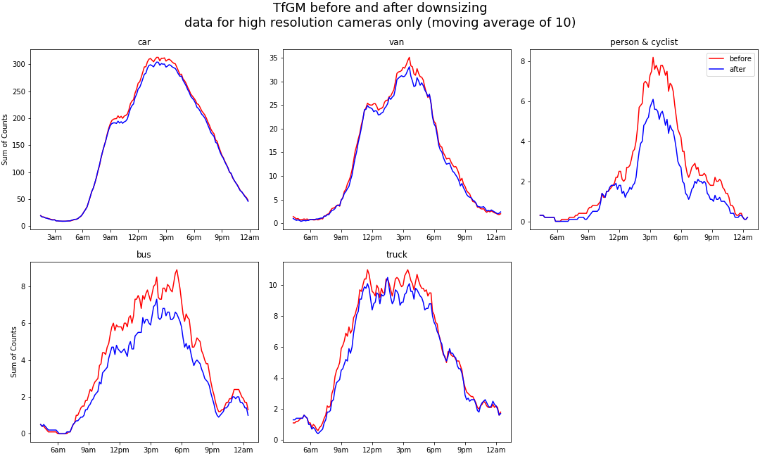
Figure 6c: Summed object counts from ‘guilty’ cameras for each 10-minute snapshot over a 24-hour period before and after downsampling for TfGM with an applied 10 period moving average
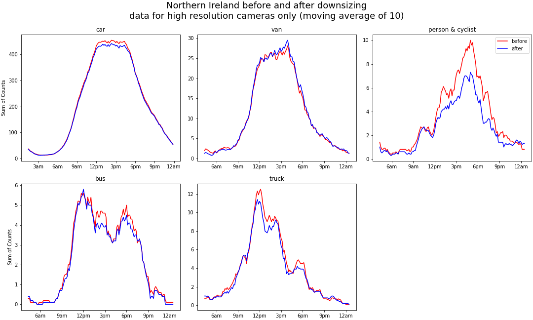
Figure 6d: Summed object counts from ‘guilty’ cameras for each 10-minute snapshot over a 24-hour period before and after downsampling for Northern Ireland with an applied 10 period moving average
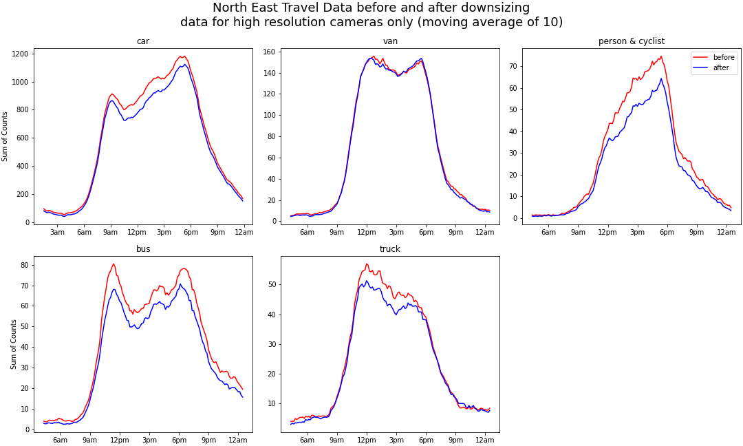
Figure 6e: Summed object counts from ‘guilty’ cameras for each 10-minute snapshot over a 24-hour period before and after downsampling for the North East with an applied 10 period moving average
When comparing object counts between “native” image resolution and downsampled resolution, we noted two main points. Firstly, downsampling higher resolution images does impact object counts for all categories and locations. Secondly, before and after counts track closely together, showing the same trends, peaks, and troughs. Before and after counts for person & cyclist and bus deviate the greatest across all locations. Generally, object counts are negatively impacted by downsampling as the blue lines trend slightly lower, with exceptions such as Southend-van, Southend-car, and Northern Ireland-van. Given that Figure 6 only shows guilty cameras, the impact on the overall counts for locations will be minimal. We investigate this further with correlation analysis, as presented in Table 2.
| Pearson Correlation | Before: Car | Before: Van | Before: Bus | Before: Truck | Before: Person/Cyclist |
|---|---|---|---|---|---|
| After: Car | 0.96 | 0.34 | 0.06 | 0.14 | 0.05 |
| After: Van | 0.34 | 0.87 | 0.08 | 0.24 | 0.05 |
| After: Bus | 0.06 | 0.05 | 0.86 | 0.10 | 0.12 |
| After: Truck | 0.14 | 0.17 | 0.15 | 0.80 | 0.01 |
| After: Person/Cyclist | 0.05 | 0.04 | 0.11 | 0.02 | 0.86 |
Table 2: Correlation table for global before and after downsampling objects counts
Table 2 demonstrates the global Pearson correlation table for all data shown in Figure 6. The high Pearsons correlation scores in Table 2 reflects the close relationship between before and after downsampling object counts in Figure 6. Globally (across all locations), car counts hold up the best with a 0.96 correlation, van second with 0.87, bus and person & cyclist tied third with 0.86, and truck with 0.80.
Conclusion
We demonstrate the implementation of a simple downsampling technique to remove legible vehicle registration plates to satisfy disclosure control checks. Furthermore, we show that time series before and after downsampling have shown significant close correlation across all locations and object types. This enables our system to simply download images into memory and immediately downsample them (discarding the higher resolution original), prior to passing on the smaller image for subsequent processing. No other sections of our analysis pipeline were impacted, and potentially disclosive images are never stored.
The full source code of the traffic cameras project is now available on GitHub (“chrono_lens”), where the system creates a Google Cloud Platform project, scaling out to process cameras as required. The system can pull publicly available imagery and records detected object counts into a BigQuery database, which is then used to generate weekly reports and a related CSV file of aggregate counts for export and further analysis.