otpConnect

#R
otpcon <- otpConnect()

This function establishes the connection to the OTP server. You will need to specify these in the parameter fields (i.e. hostname, router). See ?otpConnect for more information.

importLocationData and importGeojsonData

#R
originPoints <- importLocationData('PATH/TO/FILE')

This loads csv location data into propeR. Specify the unique ID column header using idcol="" (default is ‘name’), the latitude column using latcol="" (default is ‘lat’), the longitude column using loncol="" (default is ‘lon’), and (if needed) the postcode column using postcodecol="" (default is ‘postcode’).

The propeR package comes with some sample CSV data to be used alongside the OTP graph built using the sample GTFS and .osm files on the github repo. To load this data, run:

#R
originPoints <- importLocationData(system.file("extdata", "origin.csv", package = "propeR"))
destinationPoints <- importLocationData(system.file("extdata", "destination.csv", package = "propeR"))

The sample data shows an example of data with a latitude, longitude column (recommended) in the origin CSV file, and one with a postcode column only (works, but not recommended) in the destination CSV file. The importLocationData() function will call a separate function (postcodeToDecimalDegrees()) that converts postcode to latitude and longitude.

Note: the column lat_lon is generated automatically by importLocationData() and does not need to be manually entered.

locationValidator

#R
pointToPoint(output.dir = 'PATH/TO/DIR',
              otpcon = otpcon,
              locationPoints = originPoints,
              modes = 'WALK')

This function checks the validity of the origin and destination points. To do this the function tries to create a small isochrone around the location, and if this cannot be created, it will find the closest routable location and overwrite the latitude and longitude. This will the be saved the specified folder as a new file, which needs to be reloaded into propeR. The function is called using the following:

The above will check the validity of the locations for walking routes, including the use of public transport. To check the validity of the location for driving (e.g., town centres) change modes to equal CAR.

pointToPoint

#R
pointToPoint(output.dir = 'PATH/TO/DIR',
              otpcon = otpcon,
              originPoints = originPoints,
              originPointsRow = 2,
              destinationPoints = destinationPoints,
              destinationPointsRow = 2,
              startDateAndTime = '2019-08-18 12:00:00',
              modes = 'WALK, TRANSIT',
              mapOutput = F)

The most basic function in propeR is find the journey details for a trip with a single origin and destination.

A csv file with the following headers will be output:

origin, destination, start_time, end_time, distance_km, duration_mins, walk_distance_km, walk_time_mins, transit_time_mins, waiting_time_mins, pre_waiting_time_mins, transfers, cost, no_of_buses, no_of_trains, journey_details

The header walk_time_mins will become drive_time_mins or cycle_time_mins if modes is changed to CAR or BICYCLE, respectively. The column for cost will be ‘NA’ unless costEstimate = T is used. The field waiting_time_mins provides the total waiting time after the first leg of the journey starts (e.g., the first bus/train journey), the field pre_waiting_time_mins provides the time between the given startDateAndTime and the first leg of the journey (this cannot exceed the preWaitTime).

To output a PNG and interactive HTML leaflet map will as shown below, change the parameter mapOutput to T. For example:

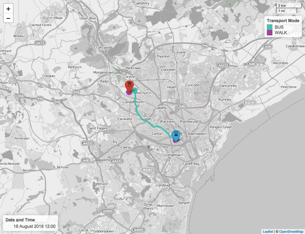
A GeoJSON of the polyline can be saved using the parameter geojsonOutput = T.

Map colours, zoom and other parameters can be specified by the user. See ?pointToPoint for details.

Note: preWaitTime is set by default to 15 minutes, any journey after this will not be deemed suitable. Please change preWaitTime value to something more appropriate, if needed.

pointToPointLoop

#R
pointToPointLoop(output.dir = 'PATH/TO/DIR',
              otpcon = otpcon,
              originPoints = originPoints,
              destinationPoints = destinationPoints,
              journeyLoop = 0,
              startDateAndTime = '2019-08-18 12:00:00',
              modes = 'WALK, TRANSIT')

This function works in the similar way to the pointToPoint() function, but instead of a single origin and destination, the function loops through all origins and/or destinations provided.

To loop just through the origins, set journeyLoop to 1, to loop just through the destinations, set journeyLoop to 2, and to loop through both, set journeyLoop to 0 (default). If you want to loop through each row of origins and route to the same row in destinations, set journeyLoop to 3. Also, you can calculate return leg journeys by setting journeyReturn to T (default is F).

pointToPointNearest

#R
pointToPointNearest(output.dir = 'PATH/TO/DIR',
              otpcon = otpcon,
              originPoints = originPoints,
              destinationPoints = destinationPoints,
              journeyReturn = F,
              startDateAndTime = '2019-08-18 12:00:00',
              modes = 'WALK, TRANSIT',
              nearestNum = 1,)

This function is useful to analyse the travel details between a destination and origin using a K-nearest neighbour (KNN) approached. It is therefore useful in analysing whether the geographically closest destination (or service) is the fastest and most appropriate for an origin.

By default k is set to 1, denoted the geographically closest destination. However, the second, third etc nearest destination can be analysed by changing the parameter nearestNum. Like pointToPointLoop the parameter journeyReturn can be used to specify whether the return journey between origin and destination should be also calculated.

pointToPointTime

#R
pointToPointTime(output.dir = 'PATH/TO/DIR',
              otpcon = otpcon,
              originPoints = originPoints,
              originPointsRow = 2,
              destinationPoints = destinationPoints,
              destinationPointsRow = 2,
              startDateAndTime = '2019-08-18 12:00:00',
              endDateAndTime = '2019-08-18 13:00:00',
              timeIncrease = 20,
              modes = 'WALK, TRANSIT',
              mapOutput = F)

This function works in the similar way to the pointToPoint() function, but instead of a single startDateAndTime, an endDateAndTime and timeIncrease (the incremental increase in time between startDateAndTime and endDateAndTime journeys should be analysed for) can be stated.

Changing mapOutput to T will save a map for each journey. To save a GIF of the time-series, set gifOutput to T. For example:

Note: if left to the default mapZoom tries to set the zoom to the bounding box ('bb') of the origin and destination locations, and the polyline created from the first API call; however, if the first call returns no journey, the map zoom level may not be appropriately set. If this is the case, you may need to manually enter an appropriate mapZoom number (e.g. mapZoom = 12).

isochrone

#R
isochrone(output.dir = 'PATH/TO/DIR',
              otpcon = otpcon,
              originPoints = originPoints,
              originPointsRow = 2,
              destinationPoints = destinationPoints,
              startDateAndTime  = '2019-08-18 12:00:00',
              modes = 'WALK, TRANSIT',
              isochroneCutOffMax = 90,
              isochroneCutOffMin = 30,
              isochroneCutOffStep = 30,
              mapOutput = F,
              geojsonOutput = F)

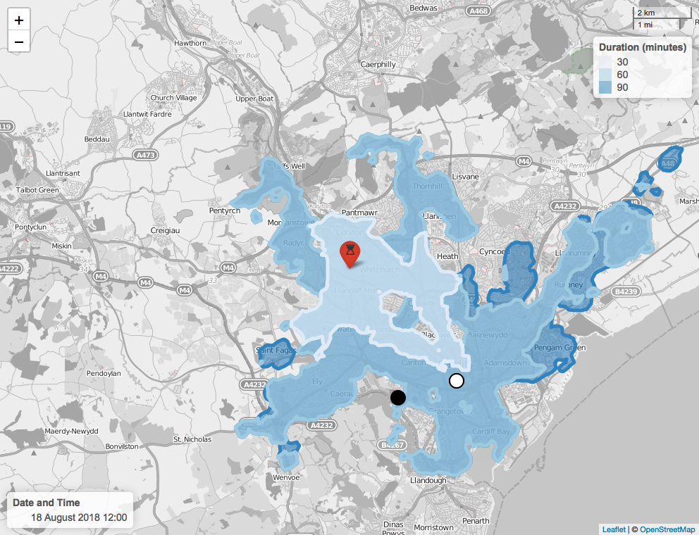
Instead of a single origin to a single destination, the isochrone function works by taking a single origin and computing the maximum distance from this origin within specified cutoff times. This means that the travel time to multiple destinations can be analysed through a single OTP API call.

A tabular output will show the travel time (in minutes) for each destination by appending the travel time to the destination from the origin to the original destination csv file. This is then saved to the specified output.dir.

A map can also be saved by usingn mapOutput = T). For example:

To save the polygon as a .GeoJSON file into the output folder, change geojsonOutput to T.

isochroneTime

#R
isochroneTime(output.dir = 'PATH/TO/DIR',
              otpcon = otpcon,
              originPoints = originPoints,
              originPointsRow = 2,
              destinationPoints = destinationPoints,
              startDateAndTime = '2019-08-18 12:00:00',
              endDateAndTime = '2019-08-18 13:00:00',
              timeIncrease = 20,
              isochroneCutOffMax = 90,
              isochroneCutOffMin = 30,
              isochroneCutOffStep = 30,
              modes = 'WALK, TRANSIT',
              mapOutput = F)

This function is to isochrone() what pointToPointTime() was to pointToPoint(), i.e., a time-series between a start and end time/date at specified time intervals that produces a table and an optional animated GIF image.

Changing mapOutput to T will save a map for each journey. To save a GIF of the time-series, set gifOutput to T. For example:

Note: if left to the default mapZoom tries to set the zoom to the bounding box ('bb') of the origin and destination locations, and the polygon created from the first API call; however, if the first call returns no journey, the map zoom level may not be appropriately set. If this is the case, you may need to manually enter an appropriate mapZoom number (e.g. mapZoom = 12).

isochroneMulti

#R
isochroneMulti(output.dir = 'PATH/TO/DIR',
              otpcon = otpcon,
              originPoints = originPoints,
              destinationPoints = destinationPoints,
              startDateAndTime  = '2019-08-18 12:00:00',
              modes = 'WALK, TRANSIT',
              isochroneCutOffMax = 90,
              isochroneCutOffMin = 30,
              isochroneCutOffStep = 30,
              mapOutput = F,
              geojsonOutput = F)

This function works similarly to the isochrone() function; however, it can handle multiple origins and multiple destinations. This is useful when considering the travel time between multiple locations to multiple possible destinations.

A PNG and interactive HTML map can also be saved in the output directory by changing mapOutput to T. For example:

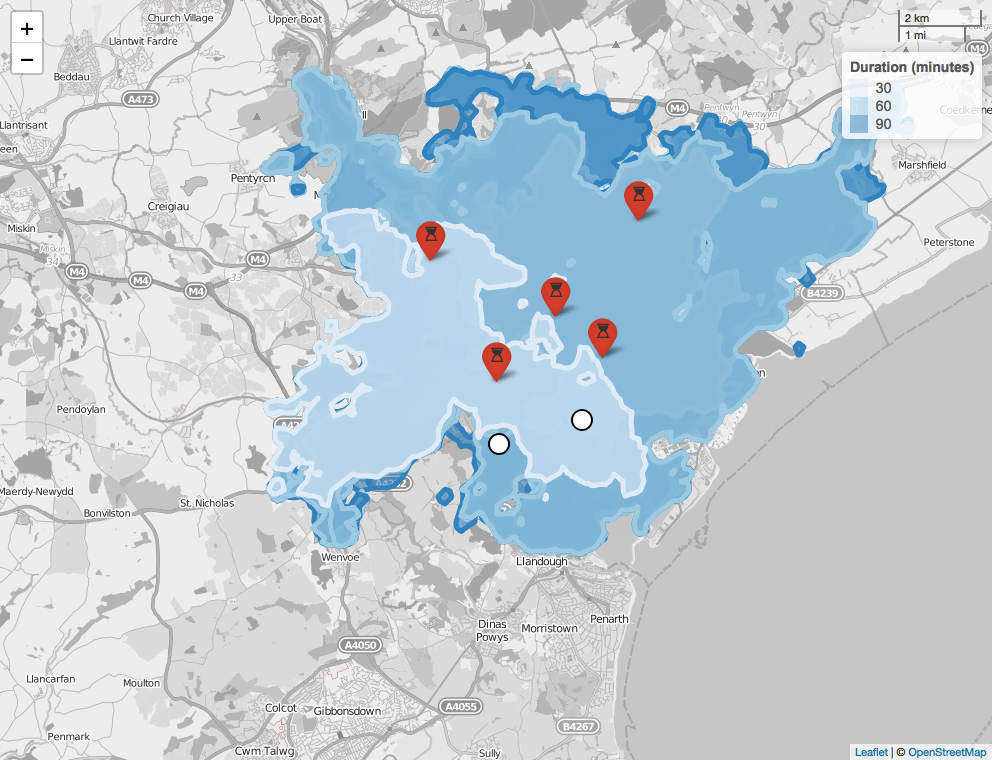
In addition, the polygons can be saved as a single .GeoJSON file by changing geojsonOutput to T.

#R
library(propeR)

Edit on GitHub