1 R
The R programming language is one of our primary tools for deriving understanding from data. The content below provides guidance on what style to use when programming and what tools we use (and recommend) to enable you to make projects more accessible and easier to share or collaborate on.
1.1 Programming Styles
Make pretty code.
Hadley Wickham’s R Style Guide should form the basis for all generated R code, this itself is based on Google’s R Style Guide. Some important points to note are to try to stick to 80 characters per line (exceptions are made for .Rmd files or similar) and to use 2 spaces, not tabs, for indentation. With regards to naming conventions, some people prefer snake_case where as others prefer camelCase; generally speaking either are fine so long as you and any collaborators are consistent with your code.
Some quick notes on what not to do when programming in R:
- Do not use
attach() - Do not use
1:length(x)when writing loops - preferseq_along() - Do not use
require(), unless you need to
Good coding style is like using correct punctuation. You can manage without it, but it sure makes things easier to read. As with styles of punctuation, there are many possible variations. The following guide describes the style that I use (in this book and elsewhere).
Good style is important because while your code only has one author, it’ll usually have multiple readers. This is especially true when you’re writing code with others. In that case, it’s a good idea to agree on a common style up-front. Since no style is strictly better than another, working with others may mean that you’ll need to sacrifice some preferred aspects of your style.
The formatR package, by Yihui Xie, makes it easier to clean up poorly formatted code. It can’t do everything, but it can quickly get your code from terrible to pretty good. Make sure to read the notes before using it.
Notation and naming
File names
File names should be meaningful and end in .R (yes, uppercase).
# Good
fit_models.R
utility_functions.R

# Bad
foo.r
stuff.r
If files need to be run in sequence, prefix them with numbers:
0_download.R
1_parse.R
2_explore.R
Pay attention to capitalization, since you, or some of your collaborators, might be using an operating system with a case-insensitive file system (e.g., Microsoft Windows or OS X) which can lead to problems with (case-sensitive) revision control systems. Never use filenames that differ only in capitalisation.
Object names
“There are only two hard things in Computer Science: cache invalidation and naming things.”
— Phil Karlton
Variable and function names should be lowercase. Use an underscore (_) to separate words within a name. Generally, variable names should be nouns and function names should be verbs. Strive for names that are concise and meaningful (this is not easy!).
Although standard R uses dots extensively in function names (contrib.url()), methods (all.equal), or class names (data.frame), it’s better to use underscores. For example, the basic S3 scheme to define a method for a class, using a generic function, would be to concatenate them with a dot, like this generic.class. This can lead to confusing methods like as.data.frame.data.frame() whereas something like print.my_class() is unambiguous.
# Good
day_one
day_1

# Bad
first_day_of_the_month
DayOne
dayone
djm1
Where possible, avoid using names of existing functions and variables. This will cause confusion for the readers of your code.
# Bad
T <- FALSE
c <- 10
mean <- function(x) sum(x)
Syntax
Spacing
Place spaces around all infix operators (=, +, -, <-, etc.). The same rule applies when using = in function calls. Always put a space after a comma, and never before (just like in regular English). There’s a small exception to this rule: :, :: and ::: don’t need spaces around them.
Place a space before left parentheses, except in a function call. Extra spacing (i.e., more than one space in a row) is ok if it improves alignment of equal signs or assignments (<-).
Do not place spaces around code in parentheses or square brackets (unless there’s a comma, in which case see above).
Curly braces
An opening curly brace should never go on its own line and should always be followed by a new line. A closing curly brace should always go on its own line, unless it’s followed by else (or a closing parenthesis).
Always indent the code inside curly braces. When indenting your code, use two spaces. Never use hard tabs (most editors allow you to replace tabs with a set number of spaces so you can still use the tab key).
It’s ok to leave very short statements on the same line:
if (y < 0 && debug) message("Y is negative")but try to avoid having more than two statements on one line
# BAD
if (y < 0 && debug) message("Y is negative"); x <- runif(10); x + 10
Pipes
If you use the %>% operator from the tidyverse, put each verb on its own line. This makes it simpler to rearrange them later, and makes it harder to overlook a step. It is ok to keep a one-step pipe in one line.
# Good
iris %>%
  group_by(Species) %>%
  summarize_all(mean) %>%
  ungroup %>%
  gather(measure, value, -Species) %>%
  arrange(value)

iris %>% arrange(Petal.Width)

# Bad
iris %>% group_by(Species) %>% summarize_all(mean) %>%
  ungroup %>% gather(measure, value, -Species) %>%
  arrange(value)
Line length
Strive to limit your code to 80 characters per line. This fits comfortably on a printed page with a reasonably sized font. If you find yourself running out of room, this is a good indication that you should encapsulate some of the work in a separate function.
Assignment
Use <-, not =, for assignment.
# Good
x <- 5

# Bad
x = 5
Quotes
Use ", not ', for quoting text. The only exception is when the text already contains double quotes and no single quotes.
Functions
- Should be verbs, where possible.
- Only use
return()for early returns. - Strive to keep blocks within a function on one screen, so around 20-30 lines maximum. Some even argue that if a function has 20 lines it should be split into smaller functions but we do not mandate this.
Commenting guidelines
Comment your code. Each line of a comment should begin with the comment (‘pound’) symbol, # and a single space: #. Comments should explain the why, not the what.
Use commented lines of - and = to break up your file into easily readable chunks.
# Load data ---------------------------
df <- read.csv('foo.csv')

# Plot data ---------------------------
ggplot(df, aes(x=foo, y=bar)) + geom_line()
1.2 Tools
The lintr package is designed to help you stick to certain coding conventions. lintr can be executed as standalone or as part of build. Using lintr will ensure we are all conforming to the same coding standards. Additionally, lintr can be ran as part of your testthat tests and integrates well with RStudio and external editors such as Emacs (with flycheck).
Quick formatting to code can be applied using the formatR package. The formatR package was designed to reformat R code to improve readability; the main workhorse is the function tidy_source(). Features include:
- long lines of code and comments are reorganized into appropriately shorter ones
- spaces and indent are added where necessary
- the number of spaces to indent the code (i.e. tab width) can be specified
- an else statement in a separate line without the leading
}will be moved one line back =as an assignment operator can be replaced with<-
Note that not all aspects of this may match the guidance we have provided above but it can at least begin to help you to refactor your code to be more accessible.
The goodpractice is useful for giving advice about good practices when building R packages. Advice includes functions and syntax to avoid, package structure, code complexity, code formatting (using lintr) and more.
1.3 Documentating Code
Documenting our code is an essential part of what we do. We should document our code to the point where someone else can view it and understand how it works and why. Documentation is also useful for future-you (so you remember what your functions were supposed to do), and for developers extending your code. When documenting functions in R, it is standard practice to use the Roxygen2 package which not only helps to generate your manual (.Rd) files, but also manages your NAMESPACE file and the Collate field of the DESCRIPTION file. This integrates really nicely with R package building. For more information on Roxygen2, see the Manual section of the R packages book and the vignettes on the CRAN package page.
1.4 Testing
In functional programming, code is designed to be reused again and again with different inputs, making for simpler code that is easier to understand and audit. Writing functions allows us to more easily document our code meaning that others can use it without too much hassle. It also means that we can build tests to ensure the code continues to work as expected when we make changes to it.
Everytime you write a new function, you should strive to write tests for that function. In fact, some people use a test driven development approach whereby tests are written first and a function is written second to pass those tests. In the case a bug is discovered with a function, a test should always be written to ensure that bug is not reintroduced at some point in the future - you are essentially protecting yourself from future you’s mistakes.
There are different packages that help with writing and running tests in R such as RUnit and testthat. It is the latter that is generally recommended. More information about testthat can be found in the R packages book.
1.5 Code Coverage
Writing tests for our code we can ensure that it works as expected and check when changes to that code break pre-existing functionality. But how do we know whether we have tested each possible scenario for our functions? How do we know which lines of code are ran during our tests? This is where code coverage comes in. Code coverage is a measure of the amount of code being exercised by a set of tests. It is an indirect measure of test quality and completeness.
For example, in the code below, we can see that lines 112-115 and 117-120 are not explicitly tested. In this case, we probably don’t need to worry very much, but on other occasions this might prompt us to write more tests.
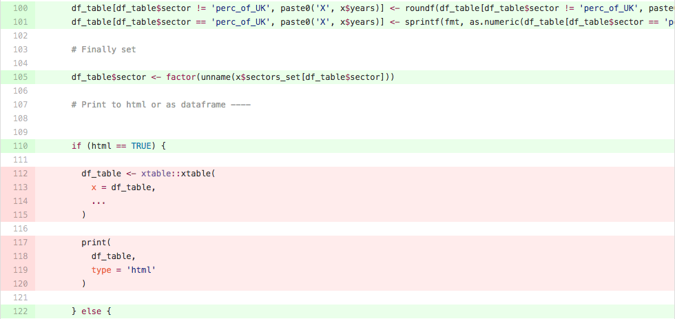
Figure 1.1: Code Coverage
Measuring code coverage allows developers to asses their progress in quality checking their own (or their collaborators) code. Measuring code coverage allows code consumers to have confidence in the measures taken by the package authors to verify high code quality. – Jim Hester
1.5.0.1 Coverage Services
In R we can obtain this functionality by using covr. This allows the user to track and report code coverage for your package and (optionally) upload the results to a coverage service like Codecov or Coveralls. covr works with both RUnit and testthat, though we are using testthat for our tests. covr provides three functions to calculate test coverage:
package_coverage()performs coverage calculation on an R package (unit tests must be contained in the “tests” directory)file_coverage()performs coverage calculation on one or more R scripts by executing one or more R scripts.function_coverage()performs coverage calculation on a single named function, using an expression provided
Please read the documentation for more information on how covr works.
1.6 Code Packaging
When writing code for a project, that code should ideally be held within a self contained package or series of packages. This helps to manage dependencies on other packages, code testing, documentation and more.
For R, there is one major resource that you should make yourself familiar with: http://r-pkgs.had.co.nz/. This book should cover all the essentials you will need to know in order to write an R package. Once you have mastered this book, you may wish to consider the Writing R Extensions manual, though this is a heavy read. When writing R packages, you should continually check the results of your R CMD check and remove any NOTEs, WARNINGs and ERRORs, where possible. We should not ship broken code!
1.7 Dependency Management
Dependency management systems are incredibly important, particularly in the world of analysis. Whenever we produce some code to perform statistical analysis or machine learning, we need to be able to recreate those results exactly. This could be the day after or the year after and we need to know which versions of which packages we must have installed on our machine. Updates to packages can produce breaking changes and our code may produce slightly different results, or worse yet, not run at all. Then installing a specific packages for a certain project may make code on other projects break.
That results can change so much with different pkg versions is scary (and ignored by many) https://t.co/wn5x3UBgQz #rstats #reproducibility pic.twitter.com/Jp4ASOKC81
— F Rodriguez-Sanchez (@frod_san) 29 March 2017
Moreover, you may be presented with someone else’s code but without them explicitly stating which packages you need, it is not always obvious, and even then you still have the manual challenge of installing the correct versions of each package yourself. These packages may then end up being globally installed when you don’t need them for any other project, therefore clogging up your system.
Whilst we would recommend docker for project management it is not always the best choice. Whilst keeping track of dependencies in R can be a chore, particularly when using lots of different packages such as those belonging to the tidyverse there are different packages which aim to help with this.
1.7.0.1 DESCRIPTION file
This is the most basic way of maintanining dependencies in R, though it is not recommended - it is only part of the dependency management system you should employ. Each R package will have a DESCRIPTION file which should contain a list of packages your package Depends on, Imports and Suggests. You can specify certain versions within for each of these.
1.7.0.2 NAMESPACE file
Dependencies in R packages are maintained using the NAMESPACE file. You should never write these files by hand as they are tedious to maintain and this approach is prone to error. Instead, you should consider using the Roxygen2 package which is detailed in the Code Documentation section of this report.
1.7.0.3 The packrat library
packrat is a dependency management system for R. Use packrat to make your R projects more:
- Isolated: Installing a new or updated package for one project won’t break your other projects, and vice versa. That’s because
packratgives each project its own private package library. - Portable: Easily transport your projects from one computer to another, even across different platforms.
packratmakes it easy to install the packages your project depends on. - Reproducible:
packratrecords the exact package versions you depend on, and ensures those exact versions are the ones that get installed wherever you go.
See the project page for more information.
1.7.0.4 The pkgsnap library
pkgsnap is a more lightweight alternative to packrat which allows you to backup and restore certain CRAN package versions. pkgsnap will create a snapshot of your installed CRAN packages with snap(), and then use restore() on another system to recreate exactly the same environment. Unfortunately pkgsnap isn’t heavily developed.